
Real-World Evidence (RWE) studies are becoming increasingly popular. Each year, the number of potential real-world data sources grows, and so does the demand for people who know how to work with them. Regulatory agencies like the FDA and EMA are publishing detailed guidance documents on RWE generation, showing that this field is definitely worth attention. RWE is already used to monitor long-term safety, assess how treatments perform in everyday care, support label expansions, meet post-marketing requirements, generate synthetic control arms for trials, drive health economics / outcomes studies, and even back up real-world performance and marketing claims. It’s also increasingly used earlier in the process to test whether a trial is feasible, find the right patients, and support recruitment strategies. Unlike clinical trials, which are slow and expensive to run, RWE studies can be done faster and at a fraction of the cost because they tap into data that’s already been collected during routine care instead of building everything from scratch.
Most resources about RWE are aimed at researchers, managers, or biostatisticians. But there’s very little practical guidance for RWE programmers or analysts, who are responsible for turning this messy, granular data into clean, analysis-ready datasets. That’s what I want to focus on here: RWE studies explained step by step, from the programmer’s point of view.
Key terms:
Before diving into workflow, it’s worth defining the most common terms. If you’re coming from a clinical trial programming background, some of these will sound familiar, but the context may be a bit different.
Real-World Data (RWD): Data collected for purposes other than clinical research. Examples: electronic health records (EHRs), insurance claims, disease registries, pharmacy data, health and wellness surveys.
Real-World Evidence (RWE): The actual conclusions drawn from RWD that support decisions about treatment, devices, or policy.
Observational / non-interventional studies: Different names for the same general concept, as opposed to clinical trials which are interventional studies, where the treatments are assigned and data is collected prospectively. In observational studies on the other hand, we analyze the data that already exists in a retrospective manner, however thare are prospective observational designs too.
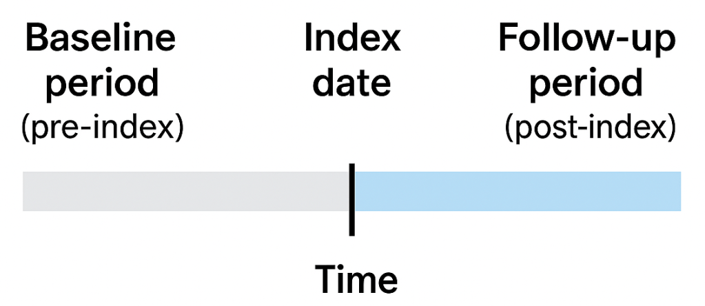
Index date: The “anchor” date for a patient. It’s often the first diagnosis of a condition, the first prescription of a drug, or the first implantation of a device. Think of it as the surrogate for “Day 1” in a clinical trial, from this date we track patient records to see what happened before and after. The other term that is related is the exposure. Basically the index date is the date when the first exposure occurs.
Baseline (pre-index) period: The time before the index date. We use it to assess patient history or his clinical status at the time of exposure – comorbidities, prior treatments, demographics.
Follow-up (post-index) period: The time after the index date. This is where we track outcomes (safety or efficacy) and measure what happens after the exposure of interest.
Cohort: The group of patients included in the study. Usually defined step by step: first, a broad initial cohort with exposure of interest selected from extremely large population of patients within a database, then narrowed down with inclusion/exclusion criteria supposed to refine the initial selection to restrict the patients to only those that are meaningful for the analysis.
Continuous enrollment / observation time: A measure that is supposed to show continuity of data available for particular patient, ensuring the patient is visible in the database over the entire period of interest. If a patient switches insurers or moves to another provider, their data may “disappear” creating gaps where we won’t be able to tell what happened to him, which can bias results.
These terms show up in almost every RWE study protocol, and as a programmer, you’ll translate them into actual logic in your code.
The RWE programming workflow, step by step:
You have to remember that unlike in clinical trials we don’t have a ready analytical dataset with relatively small, predefined number of patients in some nice predefined format. Instead we are dealing with relational database containing usually millions of patients and billions of records in a set of tables that can be linked to each other by certain key variables, and they contain only what was captured in a routine real-world medical practice with all the nuances, mistakes and missingness out there.
At a high level, almost every RWE database study follows the same pipeline. The details vary by database and research question, but the logic is remarkably consistent.
- Identify the unit of analysis
Most often, this is the patient. Sometimes, it can be events (e.g., hospitalizations, prescriptions, or procedures), with each encounter treated separately.
- Define exposure and index date
We filter the database to find patients who have the exposure of interest – usually the first diagnosis of some disease, or the first prescription of a new drug. The date of that event becomes the index date, anchoring the patient in time.
- Build the initial cohort
At this stage, the cohort is essentially a table of patient IDs and their index dates. It’s a starting point for further analysis.
- Check observation time
We need to ensure patients have continuous data during baseline and follow-up. In claims data, this is usually done by checking insurance enrollment; in EHRs, it might mean checking for continuous patient activity. If gaps exist, we either exclude the patient or acknowledge it as a study limitation.
- Derive variables
This is where programmers spend the bulk of their time. From granular event-level tables, we build patient-level variables such as:
- Demographics (age, sex, race, region, etc.)
- Clinical characteristics (comorbidities, prior drug use, Charlson Comorbidity Index, etc.)
- Outcomes of interest (hospitalization, death, treatment adherence, time-to-event measures, etc.)
- Healthcare cost and resource utilization (HCRU)
Almost nothing comes “ready-made.” For example, if you want a binary flag for diabetes at baseline, you must scan historical diagnostic codes, match them against a codelist (a list of pre-defined codes that indicate the disease – diabetes in this case), and aggregate them into a 1/0 (Yes/No) variable for each patient.
- Apply inclusion/exclusion criteria
The initial cohort is often too broad. We gradually filter it using predefined inclusion/exclusion rules (e.g., age ≥18, no prior use of the same drug, continuous observation for 12 months). At each step, we document how many patients remain. This cohort attrition flow is a critical output.
- Prepare the patient-level analysis dataset
After derivations and exclusions, we end up with a dataset that’s structured one row per patient, with derived variables in columns. This becomes the basis for statistical modeling and reporting.
- Run the analysis
At this point, the heavy lifting – cleaning, deriving, structuring the data – is complete. All that remains is to generate the output – summary tables, run some statistical tests or models, create plots – anything that is neccessary for the statistician and reasercher to make their meaningful conclusions.
Why this is challenging and fun for programmers?
Compared to clinical trial data, real-world data is messy. Diagnoses, prescriptions, and procedures are recorded for billing or operational purposes, not for research. That means:
Variables you need almost never exist directly – you have to derive them.
Data is often fragmented or incomplete.
You rely heavily on codelists and ontologies (ICD10, SNOMED, ATC, NDC, CPT – whatever the database captures) to standardize events.
Clinical input is essential (consulting the methodology with medical experts), because programmers can’t decide which codes best represent a condition and the codes may often be too general or underpopulated for some reason to clearly define the exposure. So in most cases it’s usually just the best attempt to identify the event and a judgment call on whether whether the bias is acceptable.
But that’s also what makes RWE programming engaging. It’s not just about coding tables – it’s about understanding how data is generated in real healthcare, and then engineering it into something scientifically valid.
If you are interested to know more, here are some links to useful documents about RWE in general:
- Framework for FDA’s Real-World Evidence Program
- Real-World Data: Assessing Electronic Health Records and Medical Claims Data to Support Regulatory Decision-Making for Drug and Biological Products
- Journey towards a roadmap for regulatory guidance on real-world evidence
- Real-world evidence provided by EMA
- The European Network of Centres for Pharmacoepidemiology and Pharmacovigilance (ENCePP) Guide on Methodological Standards in Pharmacoepidemiology – Revision 11
- The Book of OHDSI
- Guide to Real World Data for Clinical Research

Leave a comment